One feature I found particularly useful when adding email addresses: As you type, Excel looks through your corporate or personal address book and lists the names and addresses of contacts who match the text you’ve input. Click the address you want to add. This not only saves you a bit of time but helps make sure you don’t incorrectly type in addresses.
Next, decide whether anyone with the link can access the file, or only those whose email addresses you enter. If you see the text “Anyone with the link can edit” near the top of the pane, you can change that by clicking it, then choosing Specific people on the screen that appears. Similarly, if “Specific people” appears above the email addresses, you can change that by clicking it, then choosing Anyone with the link can edit from the screen that appears.
(If you use a business, enterprise, or education edition of Office, your IT department may have set up different sharing permissions on these two screens, such as an option to allow anyone within your organization to edit the document. You may also need to click a Link settings button — a gear icon — to access the “Link settings” pane.)
On this second screen you can also set the document to read-only for everybody, or allow everybody to edit it. In the “Other settings” section, click the down arrow and choose either Can edit, which allows full editing, or Can view, which is read-only. If you want to give certain people editing privileges and others view-only privileges, you can send two separate invitations with different rights selected.
On this screen you can also set an expiration date after which people won’t be able to access the file, and you can set a password so that only people who have the password can access it. When you’ve made your selections, click Apply.
Back in the main “Send link” screen, you can send a message along with the link by typing it into the Message box. Then click Send. An email is sent to all the recipients with a link they can click to open the document.
Your collaborators will get an email like this when you share a spreadsheet.
Preston Gralla / Foundry
(If you’d rather send recipients a copy of the file as an Excel file instead of a link, and thus not allow real-time collaboration, click Send a copy at the bottom of the “Send link” screen.)
There’s another way to share a file stored in a personal OneDrive for collaboration: In the “Copy link” area at the bottom of the “Send link” pane, click Copy. When you do that, you can copy the link and send it to someone yourself via email. Note that you have the same options for setting access and editing permissions as you do if you have Excel send the link directly for you. Just click Anyone with the link can edit or Specific people below “Copy link,” and follow the instructions above.
To begin collaborating: When your recipients receive the email and click to open the spreadsheet, they’ll open it in the web version of Excel in a browser, not in the desktop version of Excel. If you’ve granted them edit permissions, they can begin editing immediately in the browser or else click Editing > Open in Desktop App on the upper right of the screen to work in the Excel desktop client. Excel for the web is less powerful and polished than the desktop client, but it works well enough for real-time collaboration.
As soon as any collaborators open the file, you’ll see a colored cursor that indicates their presence in the file. Each person collaborating gets a different color. Hover your cursor over a colored cell that indicates someone’s presence, and you’ll see their name. Once they begin editing the workbook, such as entering data or a formula into a cell, creating a chart, and so on, you see the changes they make in real time. Your cursor also shows up on their screen as a color, and they see the changes you make.
You can easily see where collaborators are working in a shared worksheet.
Preston Gralla / Foundry
Collaboration includes the ability to make comments in a file, inside individual cells, without actually changing the contents of the cell. To do it, right-click a cell, select New Comment and type in your comment. Everyone collaborating can see that a cell has a comment in it — it’s indicated by a small colored notch appearing in the upper right of the cell. The color matches the person’s collaboration color.
To see someone’s comment in a cell, hover your cursor over the cell or put your cursor in the cell and you’ll see the comment, the name of the person who made the comment, and a Reply box you can use to send a reply. You can also click the Comments button on the upper right of the screen to open the Comments pane, which lists every comment by every person. Click any comment to jump to the cell it’s in. You can also reply when you click a comment in the pane.
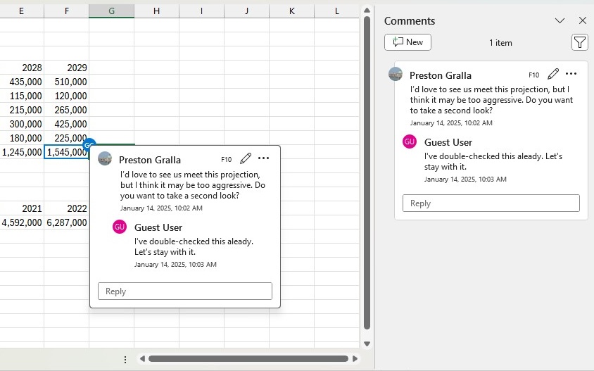
You can make see comments that other people make, and make comments yourself.
Preston Gralla / Foundry
Take advantage of linked data
Excel for Microsoft 365 has a feature that Microsoft calls “linked data types.” Essentially, they’re cells that are connected to an online source (Bing) that automatically updates their information — for example, a company’s current stock price. As I write this, there are nearly approximately 100 linked data types, including not just obvious data types such as stocks, geography, and currencies, but many others, including chemistry, cities, anatomy, food, yoga, and more.
To use them, type the items you want to track into cells in a single column. For stocks, for example, you can type in a series of stock ticker symbols, company names, fund names, etc. After that, select the cells, then on the Ribbon’s Data tab, select Stocks in the Data Types section in the middle. (If you had typed in geographic names such as countries, states, or cities, you would instead select Geography.) Excel automatically converts the text in each cell into the matching data source — in our example, into the company name and stock ticker.
Excel also adds a small icon to the left edge of each cell identifying it as a linked cell. Click any icon and a data card will pop up showing all sorts of information about the kind of information you’ve typed in. For instance, a stock data card shows stock-related information such as current price, today’s high and low, and 52-week high and low, as well as general company information including industry and number of employees. A location card shows the location’s population, capital, GDP, and so on.
You can build out a table using data from the data card. To do so, select the cells again, and an Insert Data button appears. Click the button, then select the information you want to appear, such as Price for the current stock price, or Population for the population of a geographic region.
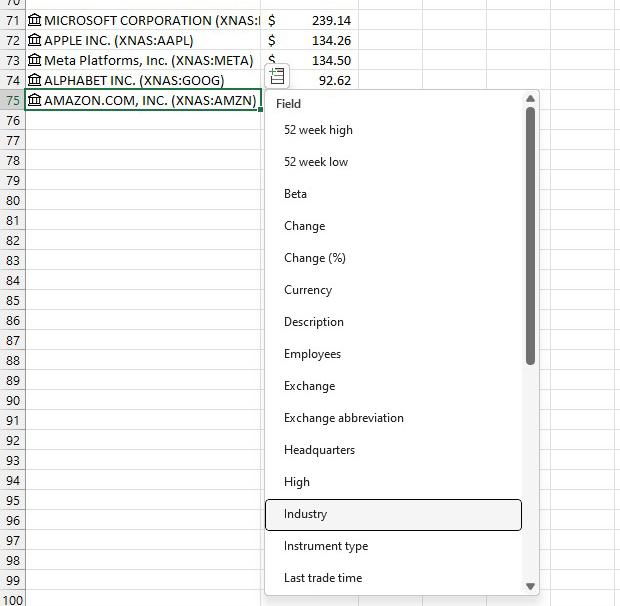
Linked data types let you insert information, such as a company’s high and low stock prices, that is continually updated.
Preston Gralla / Foundry
Excel will automatically add a column to the right populated with the latest information for each item you’re tracking, and will keep it updated. You can click the Insert Data button multiple times to keep adding columns to the right for different types of data from the item’s data card. It’s helpful to add column headers so you know what each column is showing.
Make your own custom views of a worksheet
Sheet Views let you make a copy of a sheet and then apply filtered or sorted views of the data to the new sheet. It’s useful when you’re working with other people on a spreadsheet, and someone wants to create a customized view without altering the original sheet. You can all create multiple custom-filtered/sorted views for a sheet. Once you’ve saved a sheet view, anyone with access to the spreadsheet can see it.
Note: To use this feature, your spreadsheet must be stored in OneDrive.
Sheet views work best when your data is in table format. Select the data, then go to the Ribbon toolbar and click the Insert tab. Near the left end of the Insert toolbar, click the Table button and then OK.
To create a new sheet view, click the Ribbon’s View tab, then click the New button in the Sheet View area at the far left. The row numbers and column letters at the left and top of your spreadsheet turn black to let you know you’re in a new sheet view. In the Sheet View area of the Ribbon, it says Temporary View, the default name given to a new sheet view before you’ve saved it.
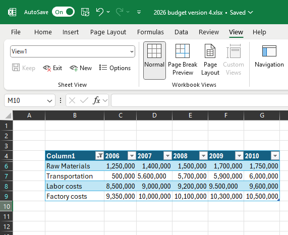
Here’s a sheet view with data sorted from highest to lowest costs.
Preston Gralla / Foundry
Now apply whatever sorting and filtering you like to the data. (If you need help, see the “How to sort and filter data” section of our Excel tables guide.)
To save this view, click the Keep button in the Sheet View area of the Ribbon. When you do that, it is saved as “View1” by default. You can click View1 and type in a more meaningful name for the view. When you click Exit on this toolbar, you return to your spreadsheet, and the row numbers and columns on the left and top of the spreadsheet are no longer black.
To switch from one sheet view to another, click the View tab. At the left of the Ribbon toolbar, click the down arrow next to the name of the current view (it will say Default if you’re viewing the spreadsheet without a sheet view applied) to open a dropdown list of the sheet views created for the spreadsheet. Click the name of a sheet view to switch to it. Whenever you’re looking at a sheet view, the row numbers and column letters framing your spreadsheet remain black to indicate that you’re in a sheet view, not the original spreadsheet.
Create dynamic arrays and charts
Dynamic arrays let you write formulas that return multiple values based on your data. When data on the spreadsheet is updated, the dynamic arrays automatically update and resize themselves.
To create a dynamic array, first create a table as outlined in the previous tip. Make sure to include a column that lists categories. Also put in at least one column to its right that lists corresponding values. Put a header at the top of each column.
So, for example, if you’re creating a spreadsheet for a business trip budget, Column A might list expenses, such as plane tickets, meals, hotel, etc., and Column B could list each item’s cost on the same row.
Once you’ve set up the table, use a dynamic array function on it, such as FILTER, SORT, or UNIQUE to create a dynamic array next to the table. Here’s an example of a formula for using the FILTER function:
=FILTER(A2:B9, B2:B9 < 2000)
This tells Excel to show only the items that cost less than $2,000 in the array.
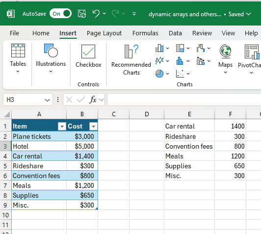
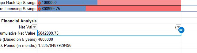
The FILTER function created a data array showing only the items with costs below $2,000.
Preston Gralla / Foundry
Now, whenever the data in your source table changes, the dynamic array updates and resizes itself to accommodate the changes. That means the dynamic array is always up to date. So in our example, if you add new items with values under $2,000 to the table, the dynamic array will enlarge itself and include those new items.
In the same way, you can use the SORT function to sort data and the UNIQUE function to remove duplicate data. (Read about more ways to use the FILTER, SORT, and UNIQUE functions from Microsoft support.)
You create a dynamic chart from the dynamic array in the same way you do any other Excel chart. Select the cells from the dynamic array that you want to chart, then select the Insert tab and select the type of chart you want to add. When the source data changes in a way that affects the dynamic array that the chart is based on, both the dynamic array and the chart will be updated.
Use AutoSave to provide a safety net as you work
If you’re worried that you’ll lose your work on a worksheet because you don’t constantly save it, you’ll welcome the AutoSave feature. It automatically saves your files for you, so you won’t have to worry about system crashes, power outages, Excel crashes and similar problems. It only works only on documents stored in OneDrive, OneDrive for Business, or SharePoint Online. It won’t work with files saved in the older .xls format or files you save to your hard drive.
AutoSave is a vast improvement over the previous AutoRecover feature built into Excel. AutoRecover doesn’t save your files in real time; instead, every several minutes it saves an AutoRecover file that you can try to recover after a crash. It doesn’t always work, though — for example, if you don’t properly open Excel after the crash, or if the crash doesn’t meet Microsoft’s definition of a crash. In addition, Microsoft notes, “AutoRecover is only effective for unplanned disruptions, such as a power outage or a crash. AutoRecover files are not designed to be saved when a logoff is scheduled or an orderly shutdown occurs.” And the files aren’t saved in real time, so you’ll likely lose several minutes of work even if all goes as planned.
AutoSave is turned on by default in Excel for Microsoft 365 .xlsx workbooks stored in OneDrive, OneDrive for Business, or SharePoint Online. To turn it off (or back on again) for a workbook, use the AutoSave slider on the top left of the screen. If you want AutoSave to be off for all files by default, select File > Options > Save and uncheck the box marked AutoSave files stored in the Cloud by default on Excel.
Using AutoSave may require some rethinking of your workflow. Many people are used to creating new worksheets based on existing ones by opening the existing file, making changes to it, and then using Save As to save the new version under a different name, leaving the original file intact. Be warned that doing this with AutoSave enabled will save your changes in the original file. Instead, Microsoft suggests opening the original file and immediately selecting File > Save a Copy (which replaces Save As when AutoSave is enabled) to create a new version.
If AutoSave does save unwanted changes to a file, you can always use the Version History feature described below to roll back to an earlier version.
Review or restore earlier versions of a spreadsheet
There’s an extremely useful feature hiding in the title bar in Excel for Microsoft 365: You can use Version History to go back to previous versions of a file, review them, compare them side-by-side with your existing version, and copy and paste from an older file to your existing one. You can also restore an entire old version.
To do it, click the file name at the top of the screen in an open file. A drop-down menu appears. Click Version History, and the Version History pane appears on the right side of the screen with a list of the previous versions of the file, including the time and date they were saved. (Alternatively, you can select the File tab on the Ribbon, click Info from the menu on the left, and then click the Version History button.)
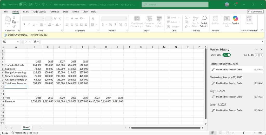
Use Version History to see all previous versions of a spreadsheet, copy and paste from an older file to your existing one, or restore an entire old version.
Preston Gralla / Foundry
In the Version History pane, click Open version under any older version, and that version appears as a read-only version in a new window. Scroll through the version and copy any content you want, then paste it into the latest version of the file. To restore the old version, overwriting the current one, click the Restore button.
Try out Microsoft 365 Copilot in Excel — but don’t expect too much
For an additional subscription fee, business users of Excel can use Microsoft’s genAI add-in, Microsoft 365 Copilot. You can have Copilot suggest and create charts, create formulas, mine spreadsheets for data insights you might have missed, and more. If you have a Microsoft 365 Personal or Family subscription, many of those features are now bundled with your core subscription.
To start using Copilot in Excel, open a spreadsheet and click the Copilot button at the right of the Ribbon’s Home tab. The Copilot panel will appear on the right, offering suggestions for actions it can perform, such as summarizing your data with a chart, adding formulas to the spreadsheet, or applying conditional formatting to the sheet. You can also chat with Copilot in the panel, asking questions about your data or how to perform an action yourself.
Note that these suggestions are generic and won’t always make sense. For example, when you start with a blank worksheet and click the Copilot button, its suggestions include summarizing data using pivot tables or charts, even though there’s no data to chart or put into a table.

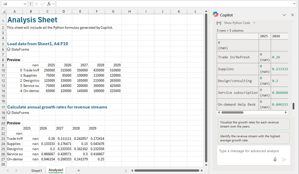
Microsoft 365 Copilot can help you in multiple ways in Excel, including creating formulas and charts, mining spreadsheets for insights, and more.
Preston Gralla / Foundry
In my testing, I found that Copilot wasn’t particularly helpful. For example, when I asked it to summarize data using a PivotTable or chart, several times it responded, “Something went wrong. Please try again in a moment.” Then it said that I first needed to reformat parts of my spreadsheet by using the Transform() function, and gave confusing advice on how I could do it — it wouldn’t do the task itself. (Eventually, I gave up.)
When I asked it to suggest conditional formatting for my spreadsheet, which would highlight important data, it told me which data I should highlight but didn’t explain why the data was important. It also didn’t do the highlighting for me or tell me how to do it.
I gave it one more try and asked it to perform an advanced analysis, which it would use Python to do. It certainly did something, although it was unclear what it was. It overwrote my original spreadsheet and added a section that claimed to show annual growth rates for revenue streams. But the data seemed to be incorrect.
Perhaps advanced spreadsheet jockeys might be able to make sense of what Copilot is up to whenever they ask it for help. But mere mortal businesspeople may find it of no help at all.
In my testing, I found Copilot not at all helpful, although spreadsheet jockeys may be able to make some sense of what it does.
Preston Gralla / Foundry
What’s more, Microsoft’s focus on Copilot in M365 has reduced the usefulness of Excel in some ways. For example, there used to be a handy feature called Smart Lookup that let you conduct targeted web searches from inside Excel. But at the beginning of 2025, Microsoft removed Smart Lookup from Excel, saying that the feature has been deprecated.
Now the only way to search the web from inside Excel is via Copilot, which lacks some features of Smart Lookup — notably the ability to highlight words or phrases in a document and trigger an automatic web search. And M365 Copilot isn’t available to business customers unless they pay the additional subscription fee.
Other features to check out
Spreadsheet pros will be pleased with several other features and tools that have been added to Excel for Microsoft 365 over the past few years, from a quick data analysis tool to an advanced 3D mapping platform.
Get an instant data analysis
If you’re looking to analyze data in a spreadsheet, the Quick Analysis tool will help. Highlight the cells you want to analyze, then move your cursor to the lower right-hand corner of what you’ve highlighted. A small icon of a spreadsheet with a lightning bolt on it appears. Click it and you’ll get a variety of tools for performing instant analysis of your data. For example, you can use the tool to highlight the cells with a value greater than a specific number, get the numerical average for the selected cells, or create a chart on the fly.
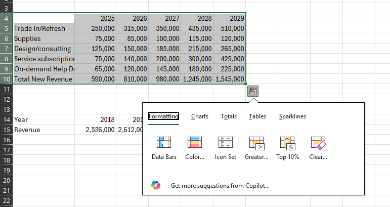
The Quick Analysis feature gives you a variety of tools for analyzing your data instantly.
Preston Gralla / Foundry
Translate text
You can translate text from right within Excel. Highlight the cell whose text you want translated, then select Review > Translate. A Translator pane opens on the right. Excel will detect the words’ language at the top of the pane; you then select the language you want it translated to below. If Excel can’t detect the language of the text you chose or detects it incorrectly, you can override it.
Easily find worksheets that have been shared with you
It’s easy to forget which worksheets others have shared with you. In Excel for Microsoft 365 there’s an easy way to find them: Select File > Open > Shared with Me to see a list of them all. Note that this only works with OneDrive (both Personal and Business) and SharePoint Online. You’ll also need to be signed into you Microsoft or work or school account.
Predict the future with Forecast Sheet
Using the Forecast Sheet function, you can generate forecasts built on historical data. If, for example, you have a worksheet showing past book sales by date, Forecast Sheet can predict future sales based on past ones.
To use the feature, you must be working in a worksheet that has time-based historical data. Put your cursor in one of the data cells, go to the Data tab on the Ribbon and select Forecast Sheet from the Forecast group toward the right. On the screen that appears, you can select various options such as whether to create a line or bar chart and what date the forecast should end. Click the Create button, and a new worksheet will appear showing your historical and predicted data and the forecast chart. (Your original worksheet will be unchanged.)
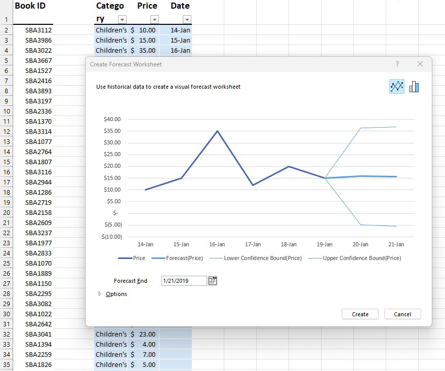
The Forecast Sheet feature can predict future results based on historical data.
Preston Gralla / Foundry
Manage data for analysis with Get & Transform
This feature is not entirely new to Excel. Formerly known as Power Query, it was made available as a free add-in to Excel 2013 and worked only with the PowerPivot features in Excel Professional Plus. Microsoft’s Power BI business intelligence software offers similar functionality.
Now called Get & Transform, it’s a business intelligence tool that lets you pull in, combine, and shape data from wide variety of local and cloud sources. These include Excel workbooks, CSV files, SQL Server and other databases, Azure, Active Directory, and many others. You can also use data from public sources including Wikipedia.
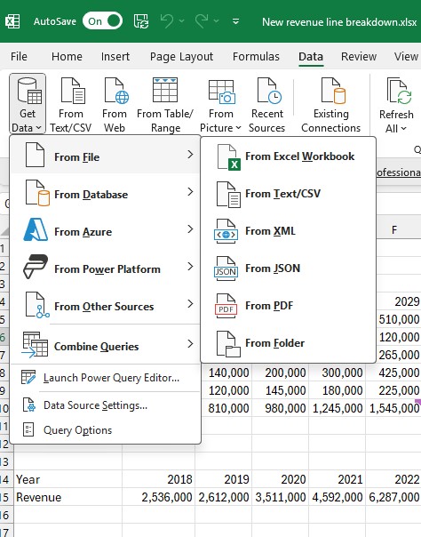
Get & Transform helps you pull in and shape data from a wide variety of sources.
Preston Gralla / Foundry
You’ll find the Get & Transform tools together in a group on the Data tab in the Ribbon. For more about using these tools, see Microsoft’s “Getting Started with Get & Transform in Excel.”
Make a 3D map
Before Excel 2016, Power Map was a popular free 3D geospatial visualization add-in for Excel. Now it’s free, built into Excel for Microsoft 365, and has been renamed 3D Maps. With it, you can plot geographic and other information on a 3D globe or map. You’ll need to first have data suitable for mapping, and then prepare that data for 3D Maps.
Those steps are beyond the scope of this article, but here’s advice from Microsoft about how to get and prepare data for 3D Maps. Once you have properly prepared data, open the spreadsheet and select Insert > 3D Map > Open 3D Maps. Then click Enable from the box that appears. That turns on the 3D Maps feature. For details on how to work with your data and customize your map, head to the Microsoft tutorial “Get started with 3D Maps.”
If you don’t have data for mapping but just want to see firsthand what a 3D map is like, you can download sample data created by Microsoft. The screenshot shown here is from Microsoft’s Dallas Utilities Seasonal Electricity Consumption Simulation demo. When you’ve downloaded the workbook, open it up, select Insert > 3D Map > Open 3D Maps and click the map to launch it.

With 3D Maps you can plot geospatial data in an interactive 3D map.
Preston Gralla / Foundry
Automate tasks
If you have OneDrive for Business and use Excel with a commercial or educational Microsoft 365 license, you can automate tasks with the Automate tab. You’ll be able to create and edit scripts with the Code Editor, run automated tasks with a button click, and share the script with co-workers. See Microsoft’s “Office Scripts in Excel” documentation for details.
Insert data from a picture into Excel
There are times you may find data inside an image file that you’d like to get into Excel. Typically, you’ll have to input the data from it manually. There’s now a way to have Excel convert the information on the image into data for a worksheet.
In the Get & Transform Data group on the Data tab, click the From Picture dropdown and select Picture From File to choose the image you want to grab data from, or Picture from Clipboard to take a screenshot of an image on your PC and then import the data. For more details, see Microsoft’s “Insert data from picture” support page.
Use keyboard shortcuts
Here’s one last productivity tip: If you memorize a handful of keyboard shortcuts for common tasks in Excel, you can save a great deal of time over hunting for the right command to click on. See “Handy Excel keyboard shortcuts for Windows and Mac” for our favorites.
This article was originally published in August 2019 and most recently updated in May 2025.
More Excel tutorials:
www.computerworld.com (Article Sourced Website)
#Excel #Microsoft #cheat #sheet